Food Insecurity Project Report

library(tidyverse)
library(gganimate)
library(kableExtra)
library(plotly)
library(readxl)
library(rvest)
library(httr)
library(RSelenium)
library(stringr)
library(usdata)


knitr::opts_chunk$set(
    echo = TRUE,
    warning = FALSE,
    fig.width = 8, 
  fig.height = 6,
  out.width = "90%"
)

theme_set(theme_minimal() + theme(legend.position = "bottom"))

options(
  ggplot2.continuous.colour = "viridis",
  ggplot2.continuous.fill = "viridis"
)

scale_colour_discrete = scale_colour_viridis_d
scale_fill_discrete = scale_fill_viridis_d

Motivation

Food Insecurity Prevalence and Significance

Food insecurity, the state of being without reliable access to a sufficient quantity of affordable, nutritious food, is a leading health and nutrition issue in the United States. In 2017 an estimated 40 million Americans (13.2 percent) were food insecure.

Food insecurity is associated with numerous adverse health outcomes, including mental health problems, diabetes, hypertension, asthma and poorer general health. As a result of the COVID-19 pandemic, millions of Americans have lost stable employment; early estimates suggest more than 50 million people, including 1 in 4 children, may be experiencing food insecurity in 2020.

Existing research has shown food insecurity to disproportionately impact non-White populations, as well as immigrants, those lacking health insurance, and those with lower educational attainment.

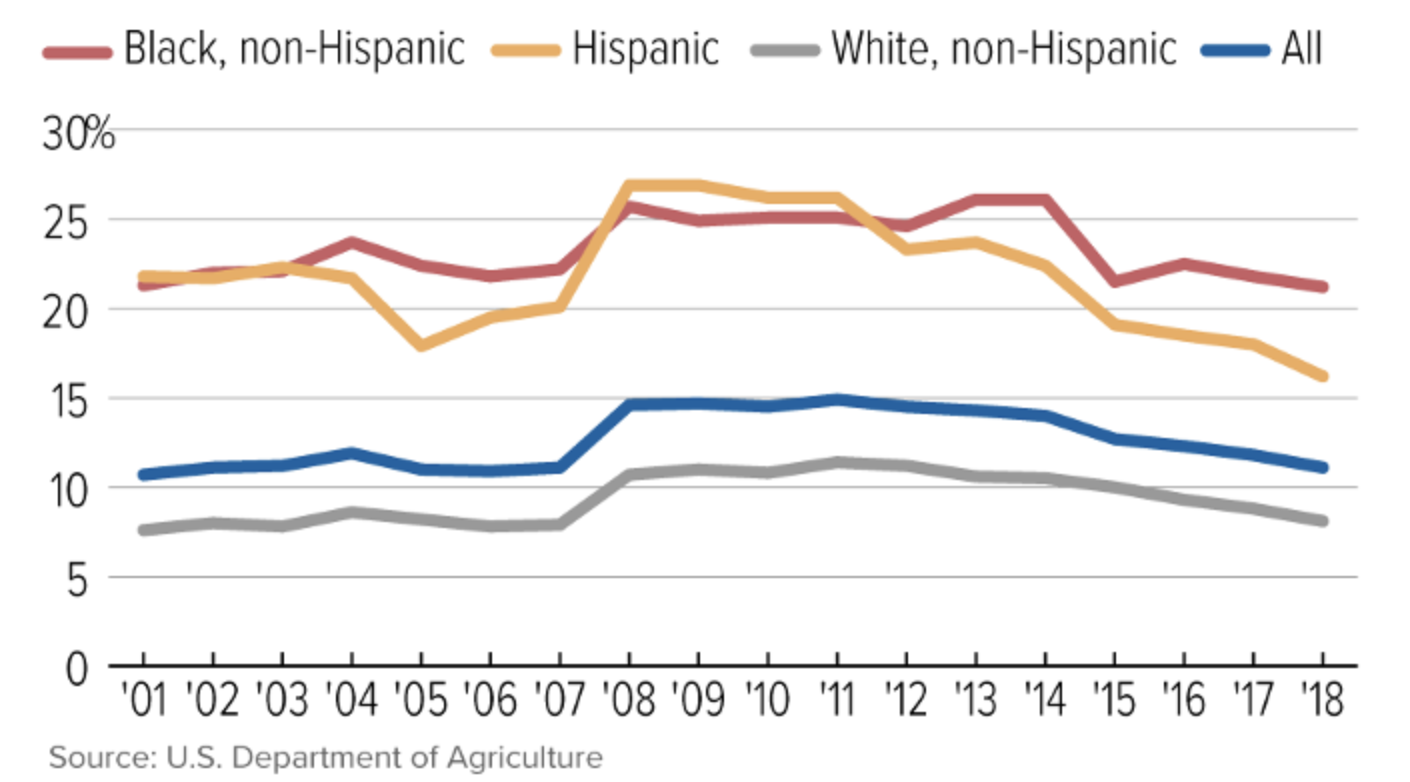
Image from Center on Budget and Policy Priorities

As a result of the increasing prevalence of food insecurity during the COVID-19 pandemic, we are collectively interested in investigating the prevalence of food insecurity on the county-level and its association with select social determinants of health.

Related Work

This is of particular importance, since research has shown the COVID-19 pandemic to be disproportionately impacting many of these same sub-populations. Moreover, a majority of food insecure individuals surveyed in Feeding America’s 2014 Hunger in America study reported having to choose between food and medical care. Increasing financial burden in 2020 due to job and/or health insurance loss may be further exacerbating this phenomenon.

Thus, identifying the specific regions and/or sub-populations at the greatest risk for food insecurity is essential to develop and enact targeted, effective intervention strategies to reduce the burden of food insecurity.

Project Questions

Initially, our overarching question was, what does the food disparity across the United States look like on national, regional, state and county levels? After investigating the variables in our datasets, we developed more specific research questions and goals, including:

• Which counties, states and regions are most disproportionately affected by food insecurity?
• What are the demographic breakdowns of food insecure counties?
• How has food insecurity changed overtime in the USA and specifically NY state?
• And, can we visualize food insecurity in an accessible way to give people information on how they can help and/or access nutrition assistance resources?

Data

We utilized Feeding America’s Map the Meal Gap data to quantify food insecurity on a county, state, regional and national level. Map the Meal Gap is an annual study conducted by Feeding America to characterize how food insecurity and food costs vary at the local level. Understanding these variations may allow communities to develop targeted strategies to reach people struggling with hunger. For this project, we used Map the Meal Gap annual study reports from years 2011 to 2019, where each report is based on US Census data from the preceding two years. Thus, the study data range from years 2009 - 2017.

Each report presents estimates of 15 food insecurity indicators generated using predictive modeling. Data were presented on the state, county, and congressional district-level. We chose to specifically focus on 8 of those 15 indicators for our analysis, which include:

• Food Insecurity Rate(the % of food insecure people)
• Number of Food Insecure Individuals
• Weighted Annual Food Budget Shortfall($)
• Cost Per Meal(Average cost per meal in $)
• Child Food Insecurity Rate(the % of food insecure children)
• Number of Food Insecure Children
• Percent of Children in Food Insecure Households with Household Incomes Below 185% of the Federal Poverty Level
• Percent of Children in Food Insecure Households with Household Incomes Above 185% of the Federal Poverty Level

As these data were contained on multiple Excel files, we used the map function to import the data across files. Since column naming was not always consistent across files, the coalesce function was used to combine data from columns representing the same variables. We then generated a unique county-state field, and re-valued select county entries using stringr to be consistent with the US Healthcare.gov Geocodes dataset county naming convention.

#import Map the Meal Gap County data using map function
path_1_df = 
tibble(
path = list.files("food_insecurity_county1_data"))

path_1_df = path_1_df %>%
  mutate(
    path = str_c("food_insecurity_county1_data/", path),
    data = map(.x = path, ~read_excel(.x))
)

path_2_df = 
tibble(
path = list.files("food_insecurity_county2_data"))

path_2_df = path_2_df %>%
  mutate(
    path = str_c("food_insecurity_county2_data/", path),
    data = map(.x = path, ~read_excel(.x, sheet = 2))
)

map_the_meal_gap_df = bind_rows(path_1_df, path_2_df)

#Fix the variable types on datasets that do not match the other datasets.
map_the_meal_gap_df[[2]][[1]]$FIPS = as.numeric(map_the_meal_gap_df[[2]][[1]]$FIPS)
map_the_meal_gap_df[[2]][[2]]$`% FI Btwn Thresholds` = as.numeric(map_the_meal_gap_df[[2]][[2]]$`% FI Btwn Thresholds`)
map_the_meal_gap_df[[2]][[1]]$`Cost Per Meal` = as.numeric(map_the_meal_gap_df[[2]][[1]]$`Cost Per Meal`)

#Unnest the data and clean names.
map_the_meal_gap_df = map_the_meal_gap_df %>%
  unnest(data) %>%
  janitor::clean_names() 

#Fix the county names to match location data and coalesce the same variables into one column.  Create an additional county_state variable to match data to location data.  Select only the new columns from coalescing.
map_the_meal_gap_df = map_the_meal_gap_df %>%
  mutate(year = str_extract(path, "_[0-9]{4}"),
         year = str_remove(year, "_"),
         state = coalesce(state_name, state),
         county_code = tolower(county_code),
         county_state = tolower(county_state),
         county = coalesce(county_code, county_state),
         county = str_replace(county, ",.*", ""),
         county = str_replace(county, "\\scounty",""),
         county = str_replace(county, "\\sparish",""),
         county = str_replace(county, "\\sborough", ""),
         county = str_replace(county, "\\scensus area", ""),
         county = str_replace(county, "\\smunicipality", ""),
         county = str_replace(county, "covington city", "covington"),
         county = str_replace(county, "do¤a ana", "doña ana"),
         county = str_replace(county, "dona ana", "doña ana"),
         county = str_replace(county, "du page", "dupage"),
         county = str_replace(county, "^st\\s|^st\\.", "saint "),
         fi_rate = coalesce(fi_rate, x2010_food_insecurity_rate, x2011_food_insecurity_rate, x2012_food_insecurity_rate, x2013_food_insecurity_rate, x2014_food_insecurity_rate, x2015_food_insecurity_rate, x2016_food_insecurity_rate, x2017_food_insecurity_rate),
         number_food_insecure_individuals = coalesce(number_food_insecure_individuals, number_of_food_insecure_persons_in_2010, number_of_food_insecure_persons_in_2011, number_of_food_insecure_persons_in_2012, number_of_food_insecure_persons_in_2013, number_of_food_insecure_persons_in_2014, number_of_food_insecure_persons_in_2015, number_of_food_insecure_persons_in_2016, number_of_food_insecure_persons_in_2017),
         child_fi_rate = coalesce(child_fi_rate, x2010_child_food_insecurity_rate, x2011_child_food_insecurity_rate, x2012_child_food_insecurity_rate, as.numeric(x2013_child_food_insecurity_rate), x2014_child_food_insecurity_rate, x2015_child_food_insecurity_rate, x2016_child_food_insecurity_rate, x2017_child_food_insecurity_rate),
         number_food_insecure_children = coalesce(number_food_insecure_children, number_of_food_insecure_children_in_2010, number_of_food_insecure_children_in_2011, number_of_food_insecure_children_in_2012, number_of_food_insecure_children_in_2013, number_of_food_insecure_children_in_2014, number_of_food_insecure_children_in_2015, number_of_food_insecure_children_in_2016, number_of_food_insecure_children_in_2017),
         cost_per_meal =
           coalesce(cost_per_meal, x2010_cost_per_meal, x2012_cost_per_meal, x2013_cost_per_meal, x2014_cost_per_meal, x2015_cost_per_meal, x2016_cost_per_meal, x2017_cost_per_meal),
         weighted_annual_dollars = na_if(weighted_annual_dollars, "n/a"),
         weighted_annual_food_budget_shortfall = coalesce(weighted_annual_food_budget_shortfall, as.numeric(weighted_annual_dollars), x2010_weighted_annual_food_budget_shortfall, x2012_weighted_annual_food_budget_shortfall, x2013_weighted_annual_food_budget_shortfall, x2014_weighted_annual_food_budget_shortfall, x2015_weighted_annual_food_budget_shortfall, x2016_weighted_annual_food_budget_shortfall, x2017_weighted_annual_food_budget_shortfall),
         percent_of_children_in_fi_hh_with_hh_incomes_below_185_percent_fpl = coalesce(percent_food_insecure_children_in_hh_w_hh_incomes_below_185_fpl,percent_of_children_in_fi_hh_with_hh_incomes_at_or_below_185_percent_fpl, percent_food_insecure_children_in_hh_w_hh_incomes_below_185_fpl_in_2012, as.numeric(percent_food_insecure_children_in_hh_w_hh_incomes_below_185_fpl_in_2013), percent_food_insecure_children_in_hh_w_hh_incomes_below_185_fpl_in_2014, percent_food_insecure_children_in_hh_w_hh_incomes_below_185_fpl_in_2015, percent_food_insecure_children_in_hh_w_hh_incomes_below_185_fpl_in_2016, percent_food_insecure_children_in_hh_w_hh_incomes_below_185_fpl_in_2017),
         percent_of_children_in_fi_hh_with_hh_incomes_above_185_percent_fpl =
           coalesce(percent_of_children_in_fi_hh_with_hh_incomes_above_185_percent_fpl, percent_of_food_insecure_children_in_hh_w_hh_incomes_above_185_fpl, percent_food_insecure_children_in_hh_w_hh_incomes_above_185_fpl_in_2012, as.numeric(percent_food_insecure_children_in_hh_w_hh_incomes_above_185_fpl_in_2013), percent_food_insecure_children_in_hh_w_hh_incomes_above_185_fpl_in_2014, percent_food_insecure_children_in_hh_w_hh_incomes_above_185_fpl_in_2015, percent_food_insecure_children_in_hh_w_hh_incomes_above_185_fpl_in_2016, percent_food_insecure_children_in_hh_w_hh_incomes_above_185_fpl_in_2017),
         ) %>%
  unite("county_state", c("county", "state"), sep = "_", remove = FALSE) %>%
  mutate(county_state = str_replace(county_state, "bristol_VA", "bristol city_VA"),
         county_state = str_replace(county_state, "dekalb_IN", "de kalb_IN"),
         county_state = str_replace(county_state, "dekalb_TN", "de kalb_TN"),
         county_state = str_replace(county_state, "dewitt_IL", "de witt_IL"),
         county_state = str_replace(county_state, "dewitt_TX", "de witt_TX"),
         county_state = str_replace(county_state, "du page_IL", "dupage_IL"),
         county_state = str_replace(county_state, "juneau city and_AK", "city and of juneau_AK"),
         county_state = str_replace(county_state, "laporte_IN", "la porte_IN"),
         county_state = str_replace(county_state, "lasalle_IL", "la salle_IL"),
         county_state = str_replace(county_state, "lasalle_LA", "la salle_LA"),
         county_state = str_replace(county_state, "matanuska susitna_AK", "matanuska-susitna_AK"),
         county_state = str_replace(county_state, "o'brien_IA", "obrien_IA"),
         county_state = str_replace(county_state, "prince georges_MD", "prince george's_MD"),
         county_state = str_replace(county_state, "queen annes_MD", "queen anne's_MD"),
         county_state = str_replace(county_state, "radford_VA", "radford city_VA"),
         county_state = str_replace(county_state, "saint  ", "saint "),
         county_state = str_replace(county_state, "saint marys_MD", "saint mary's_MD"),
         county_state = str_replace(county_state, "sainte genevieve_MO", "ste genevieve_MO"),
         county_state = str_replace(county_state, "salem_VA", "salem city_VA"),
         county_state = str_replace(county_state, "sitka city and_AK", "sitka_AK"),
         county_state = str_replace(county_state, "ste. genevieve_MO", "ste genevieve_MO"),
         county_state = str_replace(county_state, "valdez cordova_AK", "valdez-cordova_AK"),
         county_state = str_replace(county_state, " city and_AK", "_AK"),
         county_state = str_replace(county_state, "yukon koyukuk_AK", "yukon-koyukuk_AK"),
         county = county_state,
         county = str_replace(county, "_.*$", ""),
         ) %>%
  select(year, state, county, county_state, fi_rate, number_food_insecure_individuals, low_threshold_in_state, low_threshold_type, high_threshold_in_state, high_threshold_type, percent_fi_low_threshold, percent_fi_btwn_thresholds, percent_fi_high_threshold, weighted_annual_food_budget_shortfall, cost_per_meal, child_fi_rate, number_food_insecure_children, percent_of_children_in_fi_hh_with_hh_incomes_below_185_percent_fpl, percent_of_children_in_fi_hh_with_hh_incomes_above_185_percent_fpl) 

In addition to the Map the Meal Gap data, we also used 2017 US Census American Community Survey (ACS) datasets, which provide county-level breakdowns of relevant social determinants of health, including county racial and ethnic makeup, percent uninsured, percent foreign born, educational attainment breakdowns, and income category breakdowns. We merged these datasets on the county variable to generate a singular tidied table containing county-level food insecurity estimates and demographic breakdowns.

Like the Map the Meal Gap data, the ACS data were contained on multiple CSV files. Thus, we used the map function to import the data across files. To merge this dataset with the Map the Meal Gap data on the county variable, we also re-valued county entries using stringr to be consistent with the above mentioned geocodes dataset county naming convention.

#Import demographic data for 2017 using map function
path_acs_df = 
tibble(
path = list.files("ACS_data"))

acs_df = path_acs_df %>%
  mutate(
    path = str_c("ACS_data/", path),
    data = map(.x = path, ~read_csv(.x))
    ) 

#Join all the data together
acs_df = plyr::join_all(acs_df$data, by = 'GEO_ID', type = 'left') %>%
    janitor::row_to_names(1) %>%
    janitor::clean_names() %>%
    rename(county = geographic_area_name,
           estimate_total_edu_data = estimate_total,
           estimate_total_hispanic_data = estimate_total_2,
           estimate_total_immigration_data = estimate_total_3,
           estimate_total_income_data = estimate_total_4,
           estimate_total_ins_status_data = estimate_total_5,
           estimate_total_race_data = estimate_total_6) %>%
    select(id, county, starts_with("estimate"))

#Fix county strings so they match the Map the Meal Gap Data.  Add a state column and then a state_county columns.
acs_df = acs_df %>%
  mutate(county = tolower(county)) %>%
  mutate(state = str_replace(county, "^.*,", ""),
         state = state2abbr(state),
        county = str_replace(county, ",.*", ""),
         county = str_replace(county, "\\scounty",""),
         county = str_replace(county, "\\sparish",""),
         county = str_replace(county, "\\sborough", ""),
         county = str_replace(county, "\\scensus area", ""),
         county = str_replace(county, "\\smunicipality of", ""),
         county = str_replace(county, "doãƒâ±a ana", "doña ana"),
         county = str_replace(county, "^st\\s|^st\\.", "saint ")
  ) %>%
  relocate(id, county, state) %>%
  unite("county_state", c("county", "state"), sep = "_", remove = FALSE) %>%
  mutate(county_state = str_replace(county_state, "prince of wales-outer ketchikan_AK", "prince of wales-hyder_AK"))

#Join the ACS and the Map the Meal Gap data from 2017
mtm_2017_df = read_csv("./map_the_meal_gap_df.csv") %>%
  filter(year == "2017")

mtm_acs_2017_df = left_join(mtm_2017_df, acs_df, by = "county_state") %>%
  rename(state = state.x,
         county = county.x) %>%
  select(-state.y, -county.y)

#Save the csv file
write_csv(x = mtm_acs_2017_df, "mtm_acs_2017_df.csv")

In order to map these data elements onto a US county map, we also joined the zip code, latitude and longitude fields from the US Healthcare.gov Geocodes dataset onto the table. Federal Information Processing Standards (FIPS) county codes from the US Census Bureau were also separately joined onto the tidied table.

#Import location data (zip, county, longitude, and latitude) from government website.
location_data = GET("https://data.healthcare.gov/resource/geocodes-usa-with-counties.json",  query = list("$limit" = 42522)) %>% 
  content("text") %>%
  jsonlite::fromJSON() %>%
  as_tibble() 

#Fix county strings to match the Map the Meal Gap Data.  Create a county_state variable to match the data to the Map the Meal Gap Data.  
location_data = location_data %>%
  mutate(county = tolower(county)) %>%
  select(zip, state, latitude, longitude, county) %>%
  mutate(county = str_replace(county, ",.*", ""),
         county = str_replace(county, "\\scounty",""),
         county = str_replace(county, "\\sparish",""),
         county = str_replace(county, "\\sborough", ""),
         county = str_replace(county, "\\scensus area", ""),
         county = str_replace(county, "\\smunicipality of", ""),
         county = str_replace(county, "doãƒâ±a ana", "doña ana"),
         county = str_replace(county, "^st\\s|^st\\.", "saint ")
  ) %>%
  unite("county_state", c("county", "state"), sep = "_", remove = FALSE) %>%
  mutate(county_state = str_replace(county_state, "prince of wales-outer ketchikan_AK", "prince of wales-hyder_AK"))

#Save data as a csv.
write_csv(x = location_data, "location_data.csv")

#Select one zip code within a county to represent each county and save this data as a new dataframe.  Match this new dataframe to the Map the Meal Gap data (joining by county_state).
random_zip_from_county = location_data %>%
  group_by(county_state) %>%
filter(row_number() == 1)

map_the_meal_gap_df = left_join(map_the_meal_gap_df, random_zip_from_county, by = "county_state") %>%
  rename(state = state.x,
         county = county.x) %>%
  select(-state.y, -county.y) %>%
  drop_na(latitude)

#Save the new csv file.
write_csv(x = map_the_meal_gap_df, "map_the_meal_gap_df.csv")

#Import FIPS csv
#Fix county strings to match the Map the Meal Gap Data.  Create a county_state variable to match the data to the Map the Meal Gap Data.  
fips_df = readxl::read_xls("./fips_data/US_FIPS_Codes.xls", skip = 1) %>%
  janitor::clean_names() %>%
  rename(county = county_name) %>%
  unite("fips", c("fips_state", "fips_county"), sep = "") %>%
  mutate(county = tolower(county),
         state = state2abbr(state),
         county = str_replace(county, ",.*", ""),
         county = str_replace(county, "\\scounty",""),
         county = str_replace(county, "\\sparish",""),
         county = str_replace(county, "\\sborough", ""),
         county = str_replace(county, "\\scensus area", ""),
         county = str_replace(county, "\\smunicipality of", ""),
         county = str_replace(county, "dona ana", "doña ana"),
         county = str_replace(county, "^st\\s|^st\\.", "saint "),
         county = str_replace(county, "de kalb", "dekalb")
  ) %>%
unite("county_state", c("county", "state"), sep = "_", remove = FALSE) %>%
  mutate(county_state = str_replace(county_state, "prince of wales-outer ketchikan_AK", "prince of wales-hyder_AK"),
         county_state = str_replace(county_state, "matanuska susitna_AK", "matanuska-susitna_AK"),
         county_state = str_replace(county_state, "valdez cordova_AK", "valdez-cordova_AK"),
         county_state = str_replace(county_state, "juneau_AK", "city and of juneau_AK"),
         county_state = str_replace(county_state, "dekalb_TN", "de kalb_TN"),
         county_state = str_replace(county_state, "dekalb_IN", "de kalb_IN"),
         county_state = str_replace(county_state, "dewitt_IL", "de witt_IL"),
         county_state = str_replace(county_state, "de soto_MS", "desoto_MS"),
         county_state = str_replace(county_state, "de soto_FL", "desoto_FL"),
         county_state = str_replace(county_state, "du page_IL", "dupage_IL"),
         county_state = str_replace(county_state, "skagway hoonah angoon_AK", "hoonah-angoon_AK"),
         county_state = str_replace(county_state, "skagway hoonah angoon_AK", "hoonah-angoon_AK"),
         county_state = str_replace(county_state, "wrangell petersburg_AK", "petersburg_AK"),
         county_state = str_replace(county_state, "prince georges_MD", "prince george's_MD"),
         county_state = str_replace(county_state, "prince wales ketchikan_AK", "prince of wales-hyder_AK"),
         county_state = str_replace(county_state, "queen annes_MD", "queen anne's_MD"),
         county_state = str_replace(county_state, "radford_VA", "radford city_VA"),
         county_state = str_replace(county_state, "saint marys_MD", "saint mary's_MD"),
         county_state = str_replace(county_state, "yukon koyukuk_AK", "yukon-koyukuk_AK")
) %>%
  select(county_state, fips)

#Read in tidy-ed Map the Meal Gap data and join to FIPS data
map_the_meal_gap_df = read_csv("./map_the_meal_gap_df.csv")

mtm_fips_df = left_join(map_the_meal_gap_df, fips_df, by = "county_state") %>%
  drop_na(fips)

Finally a list of food banks from the Feeding America website was scraped by running a shell of the Docker software in R. We used Docker to navigate the website and unhide the data of interest, before using the CSS selector tool to identify the data’s CSS selectors. This data was also matched to the zip code, latitude and longitude data elements in order to map the food bank locations.

#Use Docker to go to the Feeding America website and scrape for the names, address/phone number, and website of 200 food banks in America. 
shell('docker run -d -p 4445:4444 selenium/standalone-chrome')
remDr <- remoteDriver(remoteServerAddr = "localhost", port = 4445L, browserName = "chrome")
remDr$open()
remDr$navigate("https://www.feedingamerica.org/find-your-local-foodbank")

list_button = remDr$findElement(using = 'css selector',"#find-fb-search-form a")
list_button$clickElement()

name_list <- remDr$findElements(using = 'css selector', ".name")
address_phone_list <- remDr$findElements(using = 'css selector', "a+ p")
website_list <- remDr$findElements(using = 'css selector', ".url a")

food_banks_df = tibble(
  name = unlist(map(name_list, function(x){x$getElementText()})),
  address_phone = unlist(map(address_phone_list, function(x){x$getElementText()})),
  website_list = unlist(map(website_list, function(x){x$getElementText()}))
)

remDr$close()

#Extract phone number and zip code from the address variable and create new columns for these two additional variables.
food_banks_df <- food_banks_df %>%
  mutate(phone_number = str_extract(address_phone, "[1-9]\\d{2}\\.\\d{3}\\.\\d{4}"),
         address_phone = str_replace(address_phone, "[1-9]\\d{2}\\.\\d{3}\\.\\d{4}", ""),
         zip = str_extract(address_phone, "\\s[0-9]\\d{4}$"),
         zip = str_replace(zip, "\\s", ""),
         address_phone = str_replace(address_phone, "\\s[0-9]\\d{4}$", ""),
         state = str_extract(address_phone, "[A-Z]{2}$")
         )

#Join the food bank data and location data.
food_banks_df = left_join(food_banks_df, location_data, by = "zip") %>%
  rename(state = state.x) %>%
  select(-state.y)

#Save the new csv file.
write_csv(x = food_banks_df, "food_banks_df.csv")

Exploratory analysis

Food insecurity and county demographic breakdowns

We created animated scatterplots joining the tidy American Community Survey data on the tidy Feeding America data to develop and compare specific variables of interest against food insecurity rates. These variables included percent race, educational attainment, insurance status, and income bracket within each county in the U.S. To compare these variables against the food insecurity rate, we converted raw counts to percents.

Using gganimate we created animated scatterplots that transition through the levels of each demographic variable with percent level on the y-axis, and food insecurity measure on the x-axis.

The below scatterplot shows the overall food insecurity rate on the x-axis by percent county breakdown of several racial groups on the y-axis.

# Create dataset containing percent of each race within each county using tidy-ed CSV file
race_per_plot =
  read_csv("mtm_2017_acs_2017_race_df.csv") %>%
    pivot_longer(
      white:hispanic,
      names_to = "race",
      values_to = "percents"
    ) %>%
    mutate(
      race = str_replace(race, "white", "White"),
      race = str_replace(race, "black", "Black"),
      race = str_replace(race, "am_ind_al_nat", "American Indian and Alaska Native"),
      race = str_replace(race, "asian", "Asian"),
      race = str_replace(race, "nat_ha_pac_isl", "Native Hawaiian and Other Pacific Islander"),
      race = str_replace(race, "other", "Other Race"),
      race = str_replace(race, "two_or_more", "Two or More Races"),
      race = str_replace(race, "hispanic", "Hispanic")
    ) %>%
    select(geo_id, total, race, percents, fi_rate) %>%
    drop_na() %>%
    ggplot(aes(x = fi_rate, y = percents, size = total, color = race)) + 
    geom_point(show.legend = FALSE, alpha = 0.8) +
    labs(
      title = '{closest_state}',
      x = "Food Insecurity Rate",
      y = "% of Individuals of Each Race"
    ) +
    theme_bw() +
    theme(text = element_text(size = 20)) +
    transition_states(race, transition_length = 1, state_length = 3, wrap = TRUE) + 
    enter_fade() + 
    exit_fade() +
    ease_aes('cubic-in-out')

## gganimate with settings
animate(race_per_plot, fps = 5, height = 500, width = 1000)

Regional variation in food insecurity

To view geographic trends in food insecurity indicators across the United States and over time, we also generated a Shiny Application using Plotly. FIPS data was used to plot the data by county. The interactive county map of the US allows users to view and compare food insecurity measures across all counties simultaneously. Users may select the food insecurity metric of interest, as well as the year and particular states, if desired.

We also created an interactive map using Leaflet which contains the locations of food banks across the United States to encourage utilization and/or donation.

To supplement the above exploratory analyses, we became interested in comparing and characterizing the prevalence of food insecurity within select New York state counties, and US states and regions. We generated animated boxplots which transition through four food insecurity indicators: overall food insecurity rate, the total number of food insecure individuals, child food insecurity rate and the number of food insecure children.

The below plot shows the overall and child food insecurity rates in select New York state counties of interest (New York, Queens, Kings, Bronx, Westchester, Albany, Saint Lawrence and Chautauqua) over the 9 year period (2009-2017):

fi_rates = 
read_csv("map_the_meal_gap_df.csv") %>%
# filter to include only counties of interest
  filter(county_state %in% c("saint lawrence_NY", "albany_NY", "chautauqua_NY", 
                             "new york_NY", "queens_NY", "kings_NY", "bronx_NY",
                             "westchester_NY")) %>%
  select(county, state, year, fi_rate, child_fi_rate) %>%
  pivot_longer(
    fi_rate:child_fi_rate,
    names_to = "rate",
    values_to = "measure"
  ) %>%
# rename values that will appear on the boxplots for easier visualization
  mutate(
    rate = str_replace(rate, "fi_rate", "Overall Food Insecurity Rate"),
    rate = str_replace(rate, "child_Overall Food Insecurity", "Child Food Insecurity Rate"),
    county = str_replace(county, "albany", "Albany"),
    county = str_replace(county, "bronx", "Bronx"),
    county = str_replace(county, "chautauqua", "Chautauqua"),
    county = str_replace(county, "kings", "Kings"),
    county = str_replace(county, "saint lawrence", "Saint Lawrence"),
    county = str_replace(county, "new york", "New York"),
    county = str_replace(county, "westchester", "Westchester"),
    county = str_replace(county, "queens", "Queens"),
    county = factor(county, levels = c("Bronx", "Kings", "Saint Lawrence", "Chautauqua", 
                                       "New York", "Queens", "Albany", "Westchester"))
    ) %>%
  # generate the boxplot through ggplot
  ggplot(aes(x = county, y = measure, color = county)) + 
  geom_boxplot(show.legend = FALSE, alpha = 0.8) +
  labs(
    title = '{closest_state}',
    x = "County",
    y = "Food Insecurity Rate"
  ) +
  theme_bw() +
  theme(text = element_text(size = 20)) +
  transition_states(rate, transition_length = 1, state_length = 3, wrap = TRUE)
# animate the boxplot to transition between the two measures: overall food insecurity and child food insecurity rates
animate(fi_rates, fps = 10, height = 500, width = 1000)

To investigate state-level food insecurity, we generated a boxplot showing overall food insecurity for each US state.

We also generated a region variable using the United States Census definitions of US regions to compare region-level food insecurity indicators. The below plot compares the overall and child food insecurity rates by US region (Northeast, South, West, Midwest) over the 9 year period (2009-2017):

# create state and region vectors
state = c("AL", "AK", "AZ", "AR", "CA", "CO", "CT", "DE", "FL", "GA", "HI", "ID", "IL",
          "IN", "IA", "KS", "KY", "LA", "ME", "MD", "MA", "MI", "MN", "MS", "MO", "MT",
          "NE", "NV", "NH", "NJ", "NM", "NY", "NC", "ND", "OH", "OK", "OR", "PA", "RI",
          "SC", "SD", "TN", "TX", "UT", "VT", "VA", "WA", "WV", "WI", "WY")
region = c("S", "W", "W", "S", "W", "W", "NE", "S", "S", "S", "W", "W", "MW", "MW", 
           "MW", "MW", "S", "S", "NE", "S", "NE", "MW", "MW", "S", "MW", "W", "MW", 
           "W", "NE", "NE", "W", "NE", "S", "MW", "MW", "S", "W", "NE", "NE", "S", 
           "MW", "S", "S", "W", "NE", "S", "W", "S", "MW", "W")
# generate a crosswalk file containing the region each state corresponds to 
x_walk = tibble(state, region)
food = read_csv("map_the_meal_gap_df.csv") 
# merge the food insecurity data with the region crosswalk
fi_rates_region = 
  merge(food, x_walk, by = "state") %>%
# rename region entries for better visualization on the generated plot
  mutate(region = str_replace(region, "MW", "Midwest"),
         region = str_replace(region, "W", "West"),
         region = str_replace(region, "NE", "Northeast"),
         region = str_replace(region, "S", "South"),
         region = factor(region, levels = c("South", "West", "Midwest", "Northeast"))
         ) %>%
  group_by(region, year) %>%
# create a mean food insecurity rate variable for each region and year
  summarize(mean_fi = mean(fi_rate), mean_child_fi = mean(child_fi_rate)) %>%
  pivot_longer(
    mean_fi:mean_child_fi,
    names_to = "mean_rate",
    values_to = "measure"
  ) %>%
  mutate(
    mean_rate = str_replace(mean_rate, "mean_fi", "Mean Food Insecurity Rate"),
    mean_rate = str_replace(mean_rate, "mean_child_fi", "Mean Child Food Insecurity Rate")) %>%
  # generate boxplot using ggplot
  ggplot(aes(x = region, y = measure, color = region)) + 
  geom_boxplot(show.legend = FALSE, alpha = 0.8) +
  labs(
    title = '{closest_state}',
    x = "Region",
    y = "Food Insecurity Measure"
  ) +
  theme_bw() +
  theme(text = element_text(size = 20)) +
  transition_states(mean_rate, transition_length = 1, state_length = 3, wrap = TRUE)
# animate plots so that they transition between mean and child food insecurity rates
animate(fi_rates_region, fps = 10, height = 500, width = 1000)

To see population-based plots depicting the number of food insecure people and children in each selected New York State county and in each US region, visit our NY and More dashboard.

After observing county, state, and region-level differences in food insecurity rates, we became interested in assessing how food insecurity may have evolved overtime in select areas. The below graph shows trends in overall food insecurity rate overtime from 2009 - 2017 in the 8 selected New York state counties of interest.

Analysis of National Trends

To visualize national trends in food insecurity, we also developed the below bar graph which shows the US food insecurity rate overtime (2009 - 2017).

read_csv("./map_the_meal_gap_df.csv") %>%
  group_by(year) %>%
  summarize(mean_fi_rate = signif(mean(fi_rate), digits = 4)) %>%
  plot_ly(x = ~year, y = ~mean_fi_rate, color = ~mean_fi_rate, type = "bar", colors = "viridis") %>%
  layout(
    title = "US National Food Insecurity Rate Over Time (2009-2017)",
    xaxis = list(title = "Year", tickfont = list(size = 10)),
    yaxis = list(title = "Food Insecurity Rate")) %>%
  colorbar(title = "Avg Food Insecurity Rate")

Discussion

Regional variation in food insecurity

There exists substantial regional variation in food insecurity and child food insecurity rates, and in the number of food insecure children and people across the United States. Through the US county map, we found that North Dakota, northern Virginia and Maryland contained counties with some of the lowest rates of food insecurity (less than 10 percent). Alabama and Mississippi, on the other hand, contained counties with some of the highest overall rates (over 35 percent).

Preliminary analysis of the box plot data showed substantial variation in food insecurity between several selected counties within New York state. We selected Kings, Bronx, New York, Queens, Westchester, Albany, Chautauqua and Saint Lawrence counties to compare food insecurity across both rural and urban communities. While the Bronx had the highest rates of overall and child food insecurity, Kings county had the largest number of food insecure individuals and children due to differences in population size. The selected rural counties (Saint Lawrence and Chautauqua) had particularly high child food insecurity rates; higher rates were observed only in Bronx county.

On a state level, Mississippi was shown to have the highest rate of overall food insecurity, while North Dakota had the lowest. Regionally, the South had the highest rates of overall and child food insecurity, as well as the greatest numbers of food insecure individuals and children. The Northeast had the lowest rates of food insecurity and fewest food insecure people.

Food insecurity and county demographic breakdowns

Observational analysis of the scatterplot data suggests that there is a difference in food insecurity rates between races, levels of educational attainment, income brackets, and insurance status.

Our results showed a positive association between percent Black race and food insecurity rate, and a negative association between percent White race and food insecurity rate on the county-level. While the vast majority of US counties contain very small percentages of American Indian and/or Alaskan Native people, there appeared to be a positive association between percent Native and food insecurity rate based on the handful of counties with large Native populations.

Among the educational attainment categories, there was a negative association between bachelor’s degree attainment and food insecurity rate. Conversely, the scatterplot showed a slight positive trend between 9-12th grade educational level and food insecurity rate. While no formal analysis was conducted, this finding is supported by the increased availability of higher paying jobs for college-educated individuals, and by the fact that college-educated individuals tend to have access to more financial resources than non-college-educated individuals.

The insurance status plots showed a positive association between percent uninsured people (ages 19-64) and food insecurity rate. Lastly, as expected, income plots showed a higher proportions of upper quartile earners were associated with reduced county-level food insecurity rate.

Trends in national food insecurity rates

The national food insecurity rate has been slowly decreasing from 2009 to 2017 from about 16.16% to about 13.24%. The average child food insecurity rate has also been decreasing, from about 25.8% to 19.36%. The average rate of child food insecurity in the USA is consistently higher than the overall average rate of food insecurity from year to year.

Correspondingly, the number of food insecure individuals in the entire USA has been slowly decreasing from 2009 to 2017 from almost 47 million (46,972,100) to just above than 40 million (40,286,060). The number of food insecure children in the entire USA has also been slowly decreasing from 2009 to 2017 from over 18 million (18,281,540) to less than 14 million (13,268,380).

The average cost per meal decreased from about $2.55 to $2.52 from 2009 to 2010 but after 2010 has been steadily increasing. In 2017 the average cost per meal was $3.02. The average weighted annual food budget shortfall in the US increased from about 6.3 million (6,325,000) in 2009 to almost 7.5 million (7,498,000) in 2014. Since 2014 the average weighted annual food budget shortfall has decreased to about 6.9 million (6,914,000) in 2017.

National Food Insecurity Metrics

Year	Avg FI Rate(%)	Avg Child FI Rate(%)	Total Num FI Indvs	Total Num FI Children	Avg Cost Per Meal	Avg Weighted Annual Food Budget Shortfall($)
2009	16.16	25.80	46972100	18281540	2.55	6325000
2010	15.57	23.10	46657180	16236840	2.52	6465000
2011	14.71	22.53	46368470	16168360	2.63	6513000
2012	14.74	22.96	45934370	16410580	2.74	7162000
2013	15.06	23.73	45744430	16615160	2.79	7400000
2014	14.68	22.81	44879260	15714050	2.89	7498000
2015	14.13	21.08	42814880	14487350	2.94	7452000
2016	13.69	20.06	41494300	13698100	3.00	7057000
2017	13.24	19.36	40286060	13268380	3.02	6914000

Overall, we found that while the national rate of food insecurity in the US has decreased from 2009 to 2017, there is still a significant percentage of the population experiencing food insecurity, and there are particular subpopulations and regions at heightened risk.

To volunteer or access nutrition assistance resources, visit Columbia University’s food pantry or Feeding America.